One of the more powerful Excel features that is relatively underused by most people – at least in my experience – is custom number formatting. It allows end users to change how numeric values are shown in the cell without changing the underlying data. This in turn enables Excel to perform calculations and link formulas to these cells, while at the same time displaying different information that better conveys its purpose.
Basic number formats are front and center in the Excel interface on the ‘Home’ tab, as they power the various options to change numbers to ‘Currency’, ‘Accounting’, ‘Percentage’, even ‘Scientific’ and ‘Date’ and ‘Time’. Ironically, I think this is partially the reason why the feature is somewhat obscure: people are using the basic version so frequently, they never think there’s a more advanced and powerful incarnation waiting to be discovered.
I won’t go into too many details about custom number formatting, as there already are excellent deep-dives on the web into its many possibilities. You can access this either from the ‘Home’ tab by clicking on the small arrow in the lower right corner next to the Number Formatting dropdown, or from the context menu of any cell by choosing ‘Format Cells…’. Then in the default ‘Number’ tab select ‘Custom’ and choose a formatting code from the list – or enter your own. Some of my favorites are these:
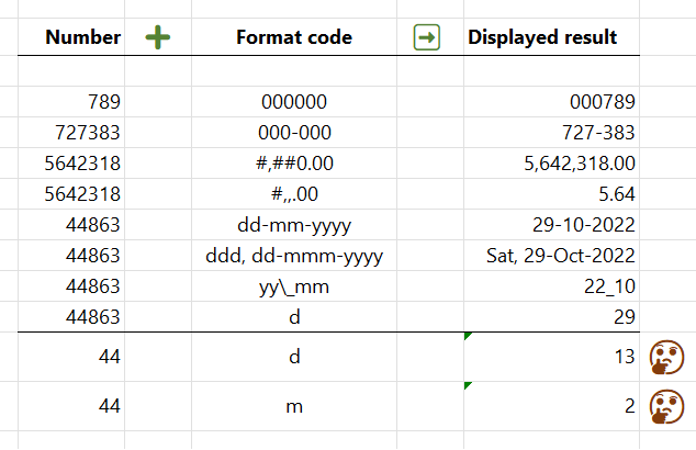
- Adding leading zeroes to numbers up until a fixed amount of digits – e.g. you need to display a 7-digit code in the cell, but some of them only have 5 or 6 digits. The format code for this is pretty straightforward: just type in as many 0s as you need! This can work to add other characters as well, such as hyphens and parentheses, which can prove useful if you want to format phone numbers.
- Rounding numbers by thousand, million, etc. – this is a code I never manage to remember, because I use it infrequently, but it provides a simple solution to round large numbers without resorting to formulas (which alter numbers by diving by a thousand/a million, so you would need to take this into account if you want to use them as basis for further calculation).
- The various date formatting combinations, which can become quite extensive. The basic codes – d for day, m for month, y for year – can be combined in multiple ways to obtain pretty much any representation of a date you need. A further note here: the repetition of these codes in a sequence also influences the end result – the more letters used, the longer the string Excel generates. This means a single d for date returns the day without a leading zero, a double d returns the day with a leading zero, a triple d the shortened name of the weekday and a quadruple d the full name of the weekday; similarly for months a single m returns the month number without a leading zero, double m returns the month with leading zero, triple m the shortened name of the month and quadruple m the full name of the month (in the language selected for the Excel locale); years are more limited with y and yy returning the last two figures and anything else the full year number.
The flexibility and complexity of the feature does come with its share of downsides though. As you may have already suspected when I mentioned rounding large numbers, custom formatting can introduce confusion if people reading the data are not familiar with the particular formatting conventions for the figures – or if the person preparing the data doesn’t properly label them.
I recently encountered a trickier case, which in turn prompted this article: a friend was using an Excel calendar template for planning at work, and added week numbers along each week row in the calendar. She was thoroughly perplexed when, for the first week of August, the week number showed… 1 instead of the correct answer, 32. I was also at first, and it took me some time to realize what was going on: the cell calculating the week number adopted the cell formatting of the neighboring cell, which was set to show a single day in the calendar with the simple d format code. But since a calendar month can have at most 31 days, this custom format resets to 1 whenever you get outside this range (in math terms, the number modulo 31), so 32 becomes 1! The month custom format has the same behavior, returning only numbers between 1 and 12. A quick reset of the formatting solved the issue of course, but it’s something to keep in mind as you use custom number formatting.
Perhaps a better solution would be for Excel to display an error if the input number is out of range in these cases. In more recent versions (Office 365 and 2021), Excel at least introduced a warning message about ‘Misleading formats’. Unfortunately this only warns about formatting of linked cells, not independent values, limiting its usefulness.

As a bonus tip, most of the standard Excel number formats can be applied via keyboard shortcuts, a combination of Ctrl, Shift, and a third key on the number row between ` to 6, as follows: Ctrl + Shift + ` turns on the ‘General’ formatting (effectively a number format reset, helpful to remember for situations like the ones described above when you want to revert to the raw number); Ctrl + Shift + 1 activates ‘Number’ (with thousand separators and two decimal places); Ctrl + Shift + 2 is for ‘Time’ and Ctrl + Shift + 3 for ‘Date’; Ctrl + Shift + 4 for ‘Currency’; Ctrl + Shift + 5 for ‘Percentage’; and finally Ctrl + Shift + 6 for default ‘Scientific’ notation. I mostly used the first two for a long time until I discovered the rest. It’s neat how some formats are cleverly aligned with related symbols on the (English) keyboard, like currency with the $ sign, percentage with % and scientific with ^, which should make it easier to remember which key applies which format.
Post a Comment